Agent Based Disease Modelling - Interactive Intro
My Masters Project: An Interactive Introduction
As part of my Masters coursework I must complete a Summer project. Partly inspired by the recent events in the world, I have chosen to do my project on Agent Based Disease Modelling.
Traditional Modelling Methods
Modern mathematical modelling is a rich subject, which informs a huge part of our lives, from weather forecasts, to bookies’ prices, to public health advice. Disease modelling is of course one area that has been in the news a great deal lately, for obvious reasons. Traditionally, mathematical modelling would fall into two, often overlapping areas. The first would be statistical modelling, fitting a distribution to some data, judging the goodness-of-fit, and using that to make predictions.
The other method, involves using calculus. Through sets of equations relating the rate of change of different quantities, scientists can study, predict and quantify aspects of a huge number of different systems and processes. These equations are called either Ordinary Differential Equations (ODEs), or Partial Differential Equations (PDEs), depending on the finer details.
In disease modelling the simplest example of this is known as the SIR model. This stands for Susceptible, Infectious, Recovered. In this model we have a population of N people. We can divided this population into groups. Those who have not had the disease, and can therefore contract it, are Susceptible. Those who currently have the disease, and can therefore spread it to others, are Infectious. Those we no longer have the disease are Recovered, this group also includes those who have died from the disease, but for this example we will assume that the disease is non lethal. We will also assume that once someone has recovered, they can no longer contract the disease again.
Having split the population into these groups, we can define relations between the groups, and model how the size of each group changes over time. These are the ODEs shown below. The values $\gamma$ and $\beta$ are constant, with $\gamma$ representing how quickly people recover from the disease, and $\beta$ representing how infectious is the disease.
$ \frac{dS}{dt} = - \frac{\beta S I}{N} $
$ \frac{dR}{dt} = \gamma I $
$ \frac{dI}{dt} = \frac{\beta S I}{N} - \gamma I $
If you are not familiar with ODEs the above equations no doubt look confusing, maybe even scary. What they are saying is actually quite simple once explained in English.
-
The first equation says that the number of Susceptible people will decrease over time, at a rate that depends on the proportion of Susceptible and Infectious people, as well as on the infectiousness of the disease.
-
The second equation says that the number of Recovered people, will increase, at a rate depending on how many Infectious people there are, as well as on how quickly people recover from the disease.
-
The third equation then says that the number of Infectious people is dependant on the proportion of Susceptible people turning Infectious, and on the number of Infectious people turning Recovered, ie. how many people are entering and leaving the Infectious group.
Mathematicians have developed different methods to study such systems. One beneficial thing we can do is use computers to numerically calculate how such a system will evolve over time. This means we start with a certain number of people in each group, as well as values for $\beta$ and $\gamma$, and see what happens to each group as time goes on. We can then plots the results.
In the two plots below we can see how the model evolved for two different values of $\beta$.
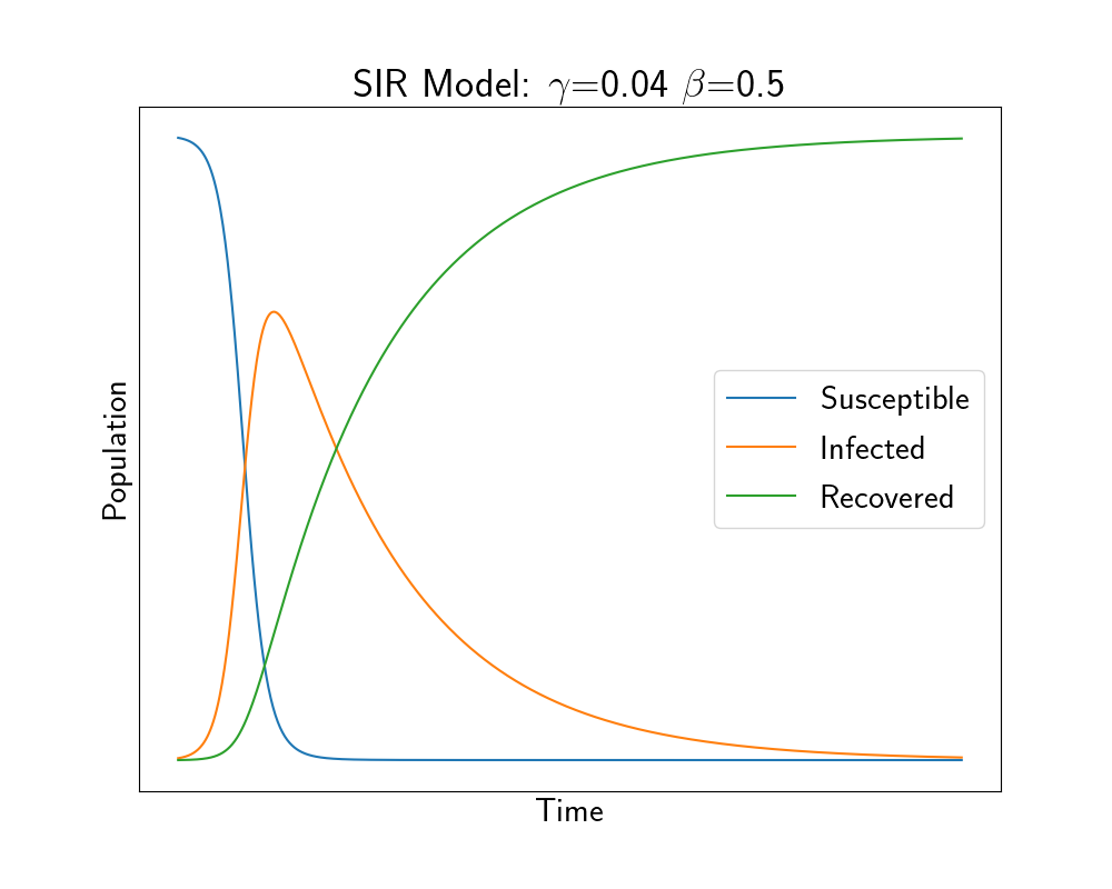
Fast Outbreak - High $\beta$
We start with most of the population being Susceptible, no one being Recovered and only a handful being Infectious. This is how most disease outbreaks would begin. We then see that the number of Infectious people skyrockets, causing Susceptible to fall, and then Recovered quickly rises as people move from being Infectious to Recovered.
When combatting a disease outbreak, one thing we usually cannot control is $\gamma$, how quickly people recover and can no longer spread the disease. One thing we can control, is $\beta$, the infectiousness of the disease. Through behaviours such as hand washing and social distancing, we can make it harder for the Infectious people to spread the disease. This is essentially lowering the $\beta$ value.
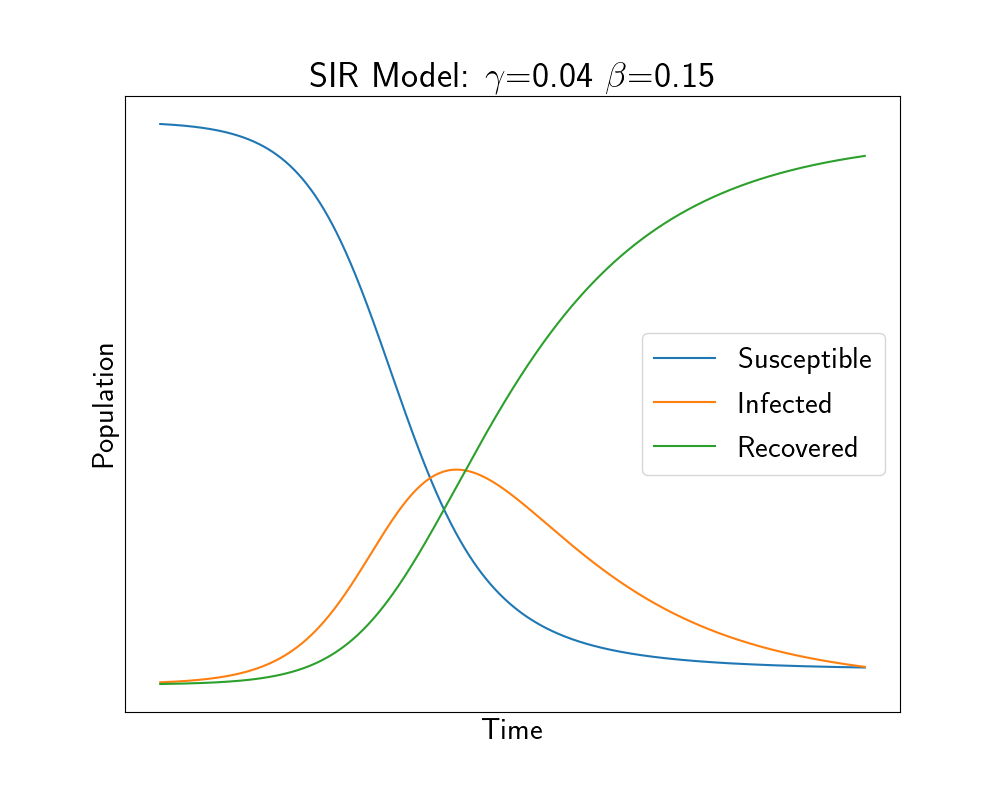
Slower Outbreak - Lower $\beta$
As we can thus see in the above plot, a lower $\beta$ means the disease spreads much more slowly. This is the “flattening of the curve” often mentioned in media.
It is incredible how such a simple model can display some of the key characteristics of disease outbreaks. And of course, such models can be extended to inlcude subtler relationships.
Agent Based Modelling
Now we can move on to the focus of my project - agent based modelling. This works in a fundamentally different way to the method outlined aboved. Instead of using equations to model the disease outbreak, we use computer simulations. In these simulations we program Agents. These agents follow rules that define how they interact with each, and with their environment.
In order to replicate the results of the SIR model, we can make the following rules.
-
Each agent will move randomly inside a given area.
-
Each agent can be either Susceptible, Infectious or Recovered.
-
If an agent is Infectious, and it comes within a certain distance of a Susceptible agent, it has a probabiltiy $\beta$ of infecting the Susceptible agent.
-
If an agent is Infectious, it has a probability $\gamma$ of becoming Recovered.
Below is an interactive implimenation of these rules. Each agent is represented by a circle bouncing in a given area. The Susceptible agents are blue, the Infectious are green and, lastly, the Recovered are red.
By playing with different values of $\gamma$ and $\beta$, you can see how quickly the circles turn from one colour to another.
Interactive Animation
Move the sliders to change the values of $\gamma$ and $\beta$. The chart below graphs the simulation in real time. By playing with the values, see the differences in the final chart.
$\gamma$ =
0.0015
$\beta$ =
0.2
Comparison
By playing around with the animation, you can see that the final plots we end up with are very similar to the plots from the traditional, equation based method. So, you might ask, if they both give similar answers, why prefer one over the other?
Both methods have their pros and cons. The equation based methods have been around much longer, and mathematician are quite good at studying equations, and can do much more with them than just the simple plotting we did above. They can mine them for a rich understanding of the underlying processes. But of course there is the famous quote;
All models are wrong, but some are useful. - George Box
Any mathematical model is a simplified version of the thing it is attempting to model. They all come with assumptions that hold to varying degrees of accuracy. In the SIR model, and most equation based disease models, a big assumption is homogenous mixing. This means we assume that everyone in the population mixes equally with everyone else in the population. Of course this helps build the model, but it is not very accurate. Humans mix within their social circles, and often have very limited contact with people outside of their circle. You are much more likely to catch a cold off your roommate than a stranger in the street.
This is something an agent based model can address. We can simply define rules for our agent that allows for heterogenous mixing. In fact, if we are clever and imaginative enough, we can define rules to address any situation we can imagine, such as social distancing, super spreaders, quarantine and vaccinations. One problem with this however, is known as verification, and it means that we must verify if the rules we have defined in our model, actually tally with what we would see in the real world.
As part of my project I am investigating and building agent based models. I thought I would share an interactive example of the simplest one, to give an idea into the differences between them and more traditional methods.